The multivariate
adaptive regression splines (MARS) were introduced by Friedman [252],[253]
as a multivariate nonparametric regression procedure. The MARS procedure fits
separate splines, which are also called basis functions, to distinct intervals
of the input variables. The basis functions have the general form:
(31)
with
BF1 as basis function, x as input
variable and a as so-called knot.
The transformation of the input variable is nonlinear, although the basis
functions are piecewise linear. A regression using two basis functions can be
described by:
(32)
with y as response variable and b0, b1 and b1
as regression coefficients. Additionally, interactions up to a prescribed
degree are also possible by the multiplication of two basis functions. The
variables, the interactions and the locations of the knots are all found by a
brute force approach and the regression coefficients are determined by a least
squares procedure. The optimal model is found by a two-step algorithm similar
to the CART principle. First, a model is grown by adding basis functions until
an overfitting occurs. In the second phase, basis functions are deleted
(pruned) until an optimal balance between overfitting and underfitting measured
by the generalized crossvalidation error (GCV) has been reached for N samples and M basis functions:
(33)
DOF (M) represents the
degrees of freedom used by the basis functions. For linear regressions, DOF (M) is usually set to M. Increasing DOF prefers smaller models.
The MARS
principle was applied to the data set of the refrigerants. The models for R22
and R134a were built by the use of the calibration data. Thereby the optimal
DOF was determined by a 10-fold crossvalidation implemented in the MARS package
[253]. The degree of allowed interaction was systematically
varied whereby the optimum for the crossvalidated calibration data was found
allowing second order interactions.
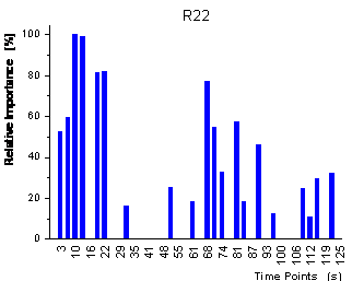
For R22,
the optimal MARS model contained 43 basis functions forming 3 additive and 27
interaction effects. In total 20 variables were used whereby the importance
of the variables is shown in figure 41 measured
by the relative amount of the reduction of the GCV by the corresponding variable.
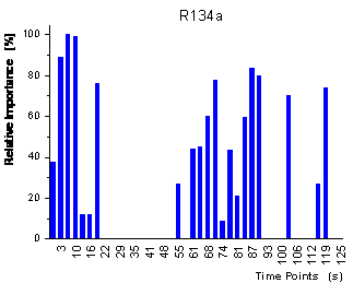
For R134a, the optimal model contained 43 basis functions forming 7 additive
and 24 interaction effects. The relative importance of the 21 variables used
by the model is also shown in figure 41. It is obvious
that for both models the relative importance of the variables is very similar
with the important variables forming two blocks after the beginning of exposure
to analyte and after the end of exposure to analyte (>60 s). These blocks
are similar to the blocks built by the CART, but in contrast to the CART both
blocks are used for both analytes.
figure 41: Relative importance
of the variables for the 2 MARS models measured by the reduction of the GCV.
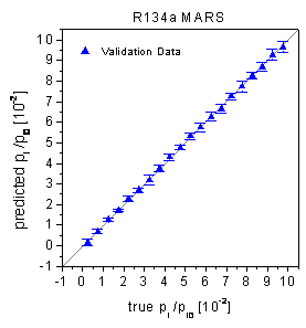
According
to table 2 the predictions of the calibration
data are very promising with relative RMSE of 1.46% for R22 and 2.27% for R134a.
The prediction errors of the validation data are significantly worse with 2.96%
for R22 and 3.71% for R134a. The rather high numbers of basis functions used
for models seem to overfit the calibration data. The true-predicted plots of
the validation data in figure 42 demonstrate that
the MARS deal well with the nonlinearities in the data and no significant bias
of the predictions can be observed in agreement with the Wald-Wolfowitz Runs
test and the Durbin-Watson statistics.
figure 42: True-predicted plots
of the MARS for the validation data.